
SASLab Manual
| |
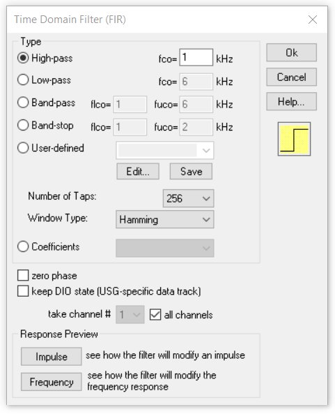
Main window : Edit > Filter > Time Domain FIR Filter
|
|
This dialog allows filtering the entire WAVE file using a Finite Impulse Response (FIR) filter.
In contrast to IIR filters, FIR filters have a finite impulse response because of their non-feedback structure, which results in a linear phase response.
The various frequency components will be delayed equally. This is a remarkable advantage over IIR filters if best fidelity of the filtered signals is required.
The drawback of FIR filters is that their execution time is longer than in IIR filters. The following filter types are available:
Type
High-pass
Removes signal components below the specified cut-off frequency (low-cut filter).
Low-pass
Removes signal components above the specified cut-off frequency (high-cut filter).
Band-pass
Keeps signal components between the specified lower and upper cut-off frequencies.
Band-stop
Removes signal components between the specified lower and upper cut-off frequencies.
The cut-off frequencies are expected in kHz and can alternatively be entered by using the measuring cursors of the spectrogram or the curve window. To do this the filter dialog box must be opened and the measuring cursors in the spectrogram or curve window must be moved to the desired location. The numeric value of the cursor is then entered automatically into the selected fields of the filter dialog box.
User-defined
This option allows selecting a predefined frequency response for the FIR filtering. The desired frequency response has to be defined in a *.flf file. In this ASCI-formatted file an unlimited number of coordinate pairs [frequency Hz] [attenuation factor] define the desired frequency response.
The frequency is specified in Hertz. The corresponding attenuation factor is a value between zero and one. It can be advantageous to edit this file in a spreadsheet application.
This is a sample of a .flf file (see also the file demo.flf in the SASLab Pro program folder):
100 0.1
200 0.3
500 0.3
2000 0.8
4000 0.1
6000 0
20000 0
Alternatively, the attenuation can also be defined in dB units (the software will interpret the data set as logarithmic dB values as soon as there is at least one negative number or the maximum is not larger than 0.0).
The Edit button below allows editing the selected frequency response file graphically. A new frequency response can be created by specifying a new file name (extension .flf). The shape of the frequency response can be edited by mouse drawing within the curve window that is launched. Existing points can be moved by left clicking and dragging them to a new location. A point can be removed by right clicking on it.
The entire shape can be removed from the drop-down menu option Edit > Reset Shape of the curve window.
The entire shape can be inverted from the drop-down menu option Edit > Invert Shape or normalized to 1.0 from Edit > Normalize Shape (use these two commands for linearizing frequency responses).
New points can be inserted by left clicking at the lines between the points.
In order to enter the modifications made in the curve window, the shape must be saved using the Save button on the Time Domain Filter (FIR) dialog box.
The resulting frequency response is then displayed in the curve window.
Number of Taps
Specifies the number of coefficients (taps) used for the filter design. More taps will produce a higher spectral resolution, which means that the width of the transition interval between the pass and stop band becomes smaller. This is however accompanied by a longer computing time.
Window Type
The FIR filter coefficients can be multiplied by a window function that is selectable here. This will reduce the ripple of the frequency response in both the pass and stop band. This is accompanied by a slight reduction of the spectral resolution.
Coefficients
This list-box allows selecting user-defined FIR coefficients. These coefficients must to be saved in a WAVE sound file with the extension .fir and the bit-depth must be 16 bit (mono). The maximum sample count (number of taps) of this file is 2048. These coefficients represent the impulse response of the filter.
Therefore this file could also be generated by recording the impulse response of a real system that is stimulated by a short pulse. In this case it may be necessary to re-scale the sound file to get the desired gain of 1.0. The factor 1.0 is represented by the integer value 32767 in the .fir file. The Coefficients must be within the range from -1.0 to 1.0 (binary -32768 to 32767).
In case the coefficients have been computed by another filter development tool, they first have to be saved in an ASCII file that can be imported into SASLab using it's ASCII import function
(File > Specials > User-defined Import Format...).
After importing the ASCII file it is necessary to save it with the extension .fir into the folder Documents > Avisoft Bioacoustics. The .fir file will then be listed in the Coefficients list box.
zero phase
This option performs zero-phase digital filtering by processing the data in both forward and reverse directions. Note that the filter is applied twice, which means that the magnitude of the original filter transfer function will be squared.
keep DIO state
If activated, this option will preserve the DIO information (related to the UltraSoundGate hardware) that is located in the least significant bit of each sample. It should only be activated when the UltraSoundGate DIO track is actually being used.
take channel #
In multichannel files, this option defines which channel will be filtered. In stereo files the left channel is referred to as channel # 1.
all channels
In multichannel files this option will filter all channels at once.
Response Preview
Impulse
This button shows the impulse response of the current filter settings in a separated curve window.
Frequency
Shows the frequency response of the current filter settings in a separated curve window.
|
|