
SASLab Manual
| |
Main window : Analyze > Specials > One-dimensional Transformation
|
|
The one-dimensional transformation tool provides additional display options and transformation types based on the marked sound file section.
The results of these transformations will be displayed in a separate curve window.
The following Functions are available:
Time signal
The fine structure of the time signal is displayed. This display allows in contrast to the envelope display on the main window a higher resolution and advanced measuring tools.
Amplitude spectrum
The magnitude spectrum (y unit [V]) of the marked section is computed. The resolution of the spectrum is proportional to the length of the marked section (long-term spectrum).
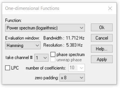
Power spectrum (logarithmic)
The power spectrum (y unit [dB]) of the marked section is computed. It is referenced to the RMS amplitude (3 dB below the peak amplitude). The phase spectrum option will add the phase spectrum in rad units and the additional option unwrap phase compensates the original phase spectrum jumps in order to provide a smooth phase spectrum.
Power spectrum (averaged)
The power spectrum (y unit [dB]) of the marked section is computed by averaging a series of short-term FFTs (50% overlap). It is referenced to the RMS amplitude (3 dB below the peak amplitude). Use this option instead of the above (Power spectrum (logarithmic)) if the time interval is very long (more than several seconds).
Power spectrum (spectrum level units)
The power spectrum (y unit spectrum level, SPL [dB]) of the marked section is computed. The SPL power spectrum is distinguished from the standard power spectrum by the term - 10 log (Bw): SPL = BL -10 log(BW), where BL is the band level of the standard power spectrum components and BW is the filter bandwidth in Hz. The spectrum level representation is useful for evaluating noise signals because the measurements are independent of the analysis bandwidth (the results are normalized to an analysis bandwidth of 1 Hz).
Power spectrum (level units, averaged)
Same as above except that the spectrum is calculated from a series of 50% overlapped short-term FFTs. Use this option instead of the above if the time interval is very long (more than several seconds).
The selectable Evaluation window will be applied to the entire marked section (except of the averaged options). With window types other than Rectangle, the signals close to the margins will be under-estimated and signals in the middle will be over-estimated. Therefore, for analyzing single pulses (with silence before and after the analysis section), the Rectangle window should be selected. This will prevent any kind of distortion, which may occur when using one of the other window types. The other non-rectangle windows should only be used if there is no silence around the margins of the marked section.
The Amplitude and Power spectrum options provide an additional LPC analysis option. The LPC option activates an additional Linear Prediction Coding procedure that is applied to the waveform before calculating the spectrogram. The LPC analysis option creates a smooth spectral envelope that indicates the major energy peaks. In primate vocalization analysis, it can help to track the formant characteristic. The number of the prediction coefficients determines the accuracy of the resulting smooth spectral envelope. The implemented LPC algorithm is based on the least-square estimation technique by using autocorrelation.
The zero padding option improves the Resolution of the spectrum by adding zeros to the selected time domain section so that the exact location of frequency peaks and magnitudes can be estimated more accurately. It does however not increase the analysis Bandwidth. The increased resolution is accomplished only by interpolating the discrete spectrum.
The selected zero padding factor (x 2 ... 128) determines the multiplication of the duration of the original time window.
Octave Analysis
The octave spectrum (y unit [dB]) of the marked section is computed by using a set of (FIR) octave filters complying with the ANSI S1.11-2004 standard. The output of the filters is linearly averaged and represents the mean RMS level. The min center frequency [Hz] list box defines the lowest octave filter. The maximum filter center frequency is determined by the sample rate of the sound file. The option include total band power adds the RMS level of the unfiltered signal to the end of the octave spectrum.
Third-Octave Analysis
The third-octave spectrum (y unit [dB]) of the marked section is computed by using a set of (FIR) 1/3 octave filters complying with the ANSI S1.11-2004 standard. The output of the filters is linearly averaged and represents the mean RMS level. The min center frequency [Hz] list box defines the lowest third-octave filter. The maximum filter center frequency is determined by the sample rate of the sound file. The option include total band power adds the RMS level of the unfiltered signal to the end of the third-octave spectrum.
Autocorrelation
The autocorrelation function (ACF) of the marked section is computed. The ACF supports the recognition of periodical or correlated components in a signal.
Cepstrum
The Cepstrum of the marked section is computed. The cepstrum is determined by calulating the inverse FFT of the logarithm of the power spectrum. Cepstral analysis supports the separation of several multiplied signal components (for instance in human speech).
Cross-correlation (stereo)
The cross correlation (CCF) between the left and right channel of the marked section of a stereo signal is computed. The CCF can be used to detect correlations between the two channels of a recording. By using two separated microphones the time delay of a noise signal can be determined by searching the maximum of the CCF.
Cross-correlation (2 files)
The cross correlation (CCF) between the marked section and the contents of the clipboard is computed. This requires that the clipboard has been loaded with the signal to be compared (Menu Edit > Copy). This kind of CCF can be used to detect similarities between two sound files.
Transfer function (2 stereo channels)
Calculates the frequency response of a system using Fourier transformation. The system input has to be supplied with a white noise signal. The left channel of the soundcard must be connected with the system input.
The right channel must be connected to the system output. After the data acquisition is finished (a few seconds are sufficient) and a subsection of the file has been marked, the computation of the transfer function is started.
Note that the marked block must be longer than the selected FFT size. If the marked section is longer, several frequency responses will be averaged, which will increase the precision, but increase the computing time.
This computation method of the frequency response provides exact results only at those frequencies, where the magnitude of the input signal is high enough. For this reason, those spectral lines of the frequency response that don't exceed a threshold within the input spectrum are suppressed in the display window.
This threshold can be changed by the slider on the right of the Curve window. This method of displaying allows using test signals that lack a continuous spectrum. One could use a rectangular signal, where valid values are only present at the frequencies f0, 3f0, 5f0, ...
Because of the algorithm used ( |G(f)|=|Sxy(f)|/|Sxx(f)| ) the frequency response is precise even if there are noise sources within the system.
Frequency response, sine sweep mono
Computes the frequency response of a system from a sine sweep test signal passing the system. It is assumed, that the test signal (sine wave with varying frequency and constant amplitude) is fed into the input of the system without distortion. The sine sweep altered by the system is then analyzed by consecutive short-time FFTs. The maximum amplitude and the frequency of that maximum are extracted from each block. The result is a frequency response plot showing amplitude against frequency. The plot is normalized relative to the maximum amplitude. The Evaluation window determines the precision of amplitude measurements. The FlatTop window is recommended for optimal results. The FFT size determines the precision of frequency measurements. High values provide more precise frequency values. However, high values will reduce the number of amplitude samples (each FFT block supplies one amplitude sample), which requires longer and slower frequency modulated test signals. An FFT size of 512 in conjunction with a test signal sweeping from 0 to the Nyquist frequency within 20 seconds is recommended. The sine sweep test signal can be generated using the command Edit/Synthesizer/dialogue.
The Incr. listbox defines the frequency axis sampling method. The default option adaptive will create a sample for each of the FFT spectra, while the other frequency options will output only provide a limited number of samples depending on the selection.
Frequency response, sine sweep stereo
Computes the frequency response of a system from a sine sweep test signal passing the system. In contrast to the function above, the test signal is sampled at both input and output of the system (using the left and right channel of a soundcard). The amplitude samples taken from the output are divided by those taken from the input. This method eliminates potential degradation caused by nonlinear test signals (varying amplitude depending on frequency). Therefore this command should also be used if it is impossible to feed the test signal into the input of the system without frequency response distortion.
In case the amplitude of the test signal is heavily attenuated by the system, an additional amplifier might be necessary. For parameter settings see the function Frequency response, sine sweep mono, described above.
Histogram
The histogram of the samples inside the marked section is computed. The number of classes can be defined dependin on the soundfile resolution (bit count).
The histogram display can be used for instance for identifying missing cides of an analog to digital converter.
XY Plot
The amplitudes of two channels are plotted against each other.
XYZ Plot
The amplitudes of three channels are plotted against each other.
Impulse density histogram
The time intervals between short signal impulses are displayed in a histogram. The detection of the signal impulses is done by a threshold comparison of the envelope of the time signal.
For the adaptation of the algorithm to the signal to be analyzed several parameters can be adjusted.
The Threshold is defined as a percentage of the maximum of the envelope. If the envelope exceeds the threshold, an impulse is recognized.
Because the impulses have a certain durations and multiple recognitions of the same impulse is undesired, a Delay time is required.
When the beginning of an impulse has been recognized, no further impulse is recognized for the delay time, even if the threshold is exceeded. The delay should be a little bit longer than the maximum impulse-width in order to prevent multiple recognitions of the same impulse.
Note that close impulses cannot be recognized if the delay is too long. The Resolution determines the tempral raster for the acquisition of the impulse density histogram.
Impulse Rate
The time intervals between short signal impulses are displayed. The detection of the signal impulses is done by a threshold comparison of the time signal.
For the adaptation of the algorithm to the signal to by analyzed several parameters can be adjusted. The Threshold is defined in percent of the maximum of the envelope.
If the time signal exceeds the threshold, an impulse is recognized (slope based). Because the impulses have certain durations and multiple recognition's of the same impulse is undesired, a Delay time is required.
When the beginning of an impulse has been recognized, no further impulse is recognized for the delay time, even if the threshold is exceeded. The delay should be a little bit longer than the maximum impulse-width to prevent multiple recognitions of the same impulse.
Note that close impulses cannot be recognized if the delay is too long.
Lorenz plot
The Lorenz plot (also called phase space display) displays the time intervals between three consecutive pulses in a 3D display. This kind of display may be useful for evaluating the randomness of pulse intervals. In constant pulse rates the Lorenz plot will display all pulses at the same location. In constantly rising or falling pulse rates, the pulses will be displayed along a straight line in 3D space.
If the pulses are more randomly spaced, the consecutive pulses will be displayed at larger distances from each other within a larger cloud in the 3D space.
The algorithm for the impulse interval measurement is the same as described for the Impulse rate function above.
Envelope (analytic signal)
The envelope of the marked section is computed. This is done by the analytical signal method using Hilbert transformation. This method allows a more precise result than the envelope display on the main window.
Instantaneous frequency
The instantaneous frequency of the marked section is computed using the analytical signal method with Hilbert transformation and differentiating filter.
The duration of the marked section is limited to 65536 samples. For isolation of separated signal sections the instantaneous frequency is displayed only if the envelope of the signal exceeds a certain value. This threshold is defined in percent of the maximum value of the whole envelope. The scroll bar on the right-hand side of the curve window allows the adjustment of the threshold.
Especially for analyzing rapidly frequency-modulated sine signals this method is advantageous compared to a spectrographic representation.
Zero-crossing analysis
A zero-crossing analysis of the marked section is carried out. The duration of the marked section is not limited. The parameter Resolution determines the temporal resolution of the output curve.
The combo box Average over allows selecting the method of averaging. By selecting the first entry (which corresponds to the Resolution edit field), the zero-crossing measurement will be averaged over that time.
By selecting one of the following entries (x cycles), the measurement will be carried out over the specified number of cycles. In that case an appropriate Resolution value should be chosen, so that temporal details will not be lost.
The implemented zero-crossing algorithm uses linear interpolation to increase the frequency resolution. For isolating separated signal sections the zero-crossing analysis is displayed only if the envelope of the signal exceeds a certain value.
This threshold is defined in percent of the maximum value of the whole envelope. The scroll bar on the right of the curve window allows the adjustment of the threshold.
Root mean square (linear) / (logarithmic)
The root mean square of the marked section is computed. The desired averaging time can be defined in the edit field Averaging time. The standard values FAST (125ms) or SLOW (1000ms) canbe retrieved from the push buttons F and S.
The option exp. determines if the averaging should be done exponentially (recursive) with the specified averaging time as time constant or arithmetically over the averaging time.
The root mean square can be displayed linear or logarithmic. For sound level measurements in dB the logarithmic root mean square should be used.
Envelope
The amplitude envelope of the marked section is computed. This is done by the following algorithm: The envelope follows the rectified waveform when its amplitude increases.
When the amplitude falls, the envelope decays with the specified Time constant, which will bridge valleys of the signal. The time constant should be adapted to the signal to be analyzed.
Gate function
This function can be used to analyze the temporal pattern of sounds. The amplitude envelope (see function above) is compared to a Threshold level. The gate function will be 1 where the amplitude envelope exceeds the threshold, and it will be zero elsewhere. The threshold is specified in percent of the maximum amplitude (measurement range). In order to tolerate short amplitude gaps or noise bursts, the gate function output will only change when the internal state of the gate function is stable for a predefined minimum time interval (the Delay parameter).
For proper operation the Delay parameter must be shorter than the minimum total duration of the pulses. The Delay parameter will also influence the temporal resolution of the gate function.
Gate function (signal/silence duration)
This function is similar to the gate function above. The only difference is the format of the output. In contrast to the above gate function that represents the output as a time-continuous sequence of ones and zeroes, this option returns the durations of the signal events and the preceding silent periods.
The y values (pulse durations) are positive for signal events, and negative for silent periods between signal events. So the output is an alternating sequence of positive event durations and negative inter-event durations, where the x-axis represents the index of the events.
Gate function (interpulse interval)
This function is similar to the Gate function (signal/silence duration), except that it provides the total time intervals between the beginnings of consecutive pulses (interpulse interval). This function is comparable to the Impulse rate function that uses a simple amplitude threshold instead of the more complex gate operation for measuring the interpulse intervals.
|
|